Toward a Panther-centered View of the Forests of South Florida

Andrew J. Kerkhoff¹, Bruce T. Milne¹, and David S. Maehr²

• Abstract
• Introduction
• Methods
  • Study area, land cover, telemetry, and sampling
  • Fractal analysis
  • Conditional mapping
• Results
• Discussion
• Speculation
  • Toward a panther-centered view
• Conclusion
• Responses to this Article
• Acknowledgments
• Literature Cited
• Appendix 1

Anthropogenic habitat degradation and loss is the single largest threat to the endangered Florida panther, Puma concolor coryi. Conservation of the subspecies must be undertaken on the scale of the entire landscape. Thus, a view of the forested landscape of South Florida must be developed that is meaningful with reference to the panther. We approach this problem by analyzing the spatial interactions of panthers and forests at multiple scales. We apply tools derived from fractal geometry to the analysis of 12 years of telemetry observations of panthers and remotely sensed forest cover imagery. A fractal characterization extends conventional scale-dependent measures of forest density and relates intuitively to panther ecology. To move toward a panther-centered view of the forests of South Florida, we adopt a scale-dependent notion of association and compare the density of forest cover associated with panther locations to that of the forest at large. Panthers interact with forest cover over a wide range of scales, consistently selecting denser than average forest areas. We discuss landscape-scale management of the panther in light of our findings and propose a protocol for mapping forest cover with reference to the panther at multiple scales as a mangement tool for habitat assessment.

KEY WORDS: Puma concolor coryi, Florida panther, anthropogenic disturbance, conditional mapping, controls on distribution, fractal analysis, habitat selection, landscape conservation, organism-centered landscapes, scale dependence, telemetry.

Published: February 3, 2000

The conservation of species in the face of habitat loss and fragmentation necessitates the study of broad ecological landscapes (Clark et al. 1993, Mladenoff et al. 1995, Maehr and Cox 1995, Keitt et al. 1997). The Florida panther, Puma concolor coryi, is a case in point. Widespread and increasing anthropogenic habitat loss is the single largest threat to the subspecies (Maehr et al. 1991, Cox et al. 1994, Maehr and Cox 1995), and the sizable home range requirements of individual panthers (Maehr et al. 1991) make the conservation of a viable population a regional, rather than local, problem. Extensive forested landscapes are critical to panther survival (Belden et al. 1988, Maehr et al. 1991, Maehr and Cox 1995), and areas preserved for panther conservation may thus encompass the habitats of many of South Florida's other rare species, both animal and plant (Kautz et al. 1993, Cox et al. 1994).

The distribution of panthers in the landscape, like ecological patterns in general, is generated by multiple biotic and abiotic processes operating on many spatial and temporal scales (Delcourt et al. 1982, Urban et al. 1987, Holling 1992, Levin 1992). Panthers respond to environmental factors over scales ranging from the regional climatic and anthropogenic controls on land cover (Maehr and Cox 1995) to the more localized biotic interactions of foraging, mating, and kitten rearing (Maehr et al. 1991). Properties of such multiscale patterns vary with the scale of observation (Meentemeyer 1989, Milne 1991, Levin 1992), reflecting the influence of different processes at different scales. Examination of the distribution of panther habitat at multiple spatial scales may thus lead to a more robust understanding of the implications of alternative management scenarios for the panther's long-term survival.

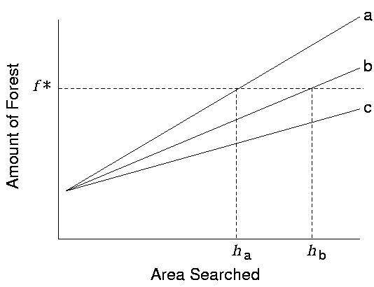
The scale dependence of the interaction between panthers and the forest becomes clear if one considers a panther on the landscape, working to balance caloric gain and metabolic costs. Forest cover is a reasonable surrogate for useful habitat, as it provides forage (deer and other prey species), potential access to mates, and shelter (both day rest and denning sites), and thus impacts fitness (Maehr et al. 1991). To ensure survival, a home range must contain some minimal amount of forest cover. In habitat-poor landscapes, panthers must range more widely, a notion supported by the observation that panther home range size is inversely related to the extent of forest cover within it (Maehr and Cox 1995). Presumably, a panther increases its home range area until it gains a sufficient quantity of resources. The distribution of forest cover determines the rate at which a panther accumulates resources as it moves about a particular landscape. Of course, some upper limit must also exist above which the maintenance of a home range becomes untenable due to metabolic travel costs. If the landscape does not provide sufficient resources at a scale below this upper limit, it is not viable as panther habitat (Fig. 1).

Fig. 1. Hypothetical relationship between available forest cover and area searched by a panther in three hypothetical landscapes (a, b, c), where f* is the threshold amount of forest necessary to support a panther. The points h correspond to the size of panther home ranges in landscapes (a) and (b). Landscape (c) fails to provide enough forest for panther maintenance.

This study is an attempt to develop a panther-centered view of the forest of South Florida (sensu Turner and Gardner 1991) by examining remotely sensed forest cover data and radio-telemetered panther locations over a wide range of spatial scales. Interpreting the managed landscape of South Florida with specific reference to panthers is critical to their conservation and to their use as an "umbrella" species under which other conservation efforts may be undertaken (Cox et al. 1994). Specifically, a panther-centered view is necessary for estimating currently available habitat and prospecting both Florida and other parts of the southeastern United States for potential reintroduction sites (Jordan 1997).

To this end, we first use a formalism derived from fractal geometry (Mandelbrot 1982, Voss 1988, Milne 1992) to describe how the area of forest cover changes with the scale of observation. Using increases in scale as a surrogate for increases in search area, we predict that panthers favor those landscapes that provide the greatest gain in forest area for a given increase in scale. Next, we assess the association of forest cover and panther locations at multiple scales via conditional mapping (Scheuring and Riedi 1994, Milne 1997). We hypothesize that the subset of forest associated with panther locations will exhibit denser aggregation than the forest as a whole, reflecting panther habitat selection. We then address landscape-scale panther management in light of our findings. Finally, we provide a method for mapping forest density at multiple scales with specific reference to panther preferences. This approach may account for the ecological choices made by animals at multiple spatial and temporal scales (Senft et al. 1987, Holling 1992).

Study area, land cover, telemetry, and sampling

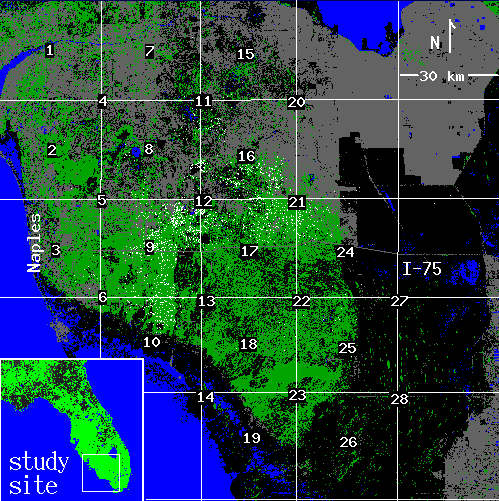
The study area consisted of approximately 20,000 km² of South Florida (Fig. 2), encompassing the currently occupied range of the Florida panther. About 22% (4300 km²) of the area is forested, mostly occurring toward the coast of the Gulf of Mexico, northwest of the Everglades. A more complete site description is available from Maehr and Cox (1995). Land cover maps were based on 1986-1989 Landsat Thematic Mapper imagery, with a 30-m pixel resolution. One pixel of forest corresponds to 900 m² of forest cover. Classification and verification procedures and class descriptions are provided by Kautz et al. (1993). Forest cover was represented by five classes, all of which serve as critical panther habitat (Maehr et al. 1991, Maehr and Cox 1995): hardwood hammock, cypress swamp, hardwood swamp, pinelands, and mixed hardwood-pine. All other classes were simply considered nonforest.

Fig. 2. South Florida study area, encompassing the currently occupied range of the Florida panther. Forest areas are green. Human-dominated areas (barren, urban, agricultural, rangeland) are gray. Panther locations are white. Black areas are primarily perennial wetlands, which are avoided by panthers. Numbers correspond to the center of each 30 x 30 km study plot.

Panther telemetry locations (N = 12,783) were obtained by the Florida Game and Freshwater Fish Commission three times per week from February 1981 to November 1993 (Maehr et al. 1991, Maehr and Cox 1995) and were mapped to the nearest 100 m. Each collared panther was located at least once on every flight. We compiled two binary (presence/absence) maps, one of forest cover and one of panther locations. Because the subject of this study was the overall relationship between the panther population and forest cover, we made no distinction between the five forest cover classes, nor between telemetry locations representing the 41 individual panthers, nor between those locations visited by panthers once and those visited many times.

We divided the study area into a uniform grid of 900 km² (1000 x 1000 pixel) plots. Because our analyses concentrate on approximately the center one-half of each plot, a second grid of plots was overlaid on the first and offset so that the center of each new plot corresponded to an intersection in the original grid (Fig. 2). In this way, most of the landscape was subject to analysis, with negligible overlap between areas from which statistics were obtained. In all plots, we tabulated the number of panther locations and calculated percent forest cover. We omitted plots with less than 3% forest cover, which yielded 28 plots. In subsequent analyses, we examined the subset of forest associated with panther locations. To ensure the presence of resident animals, we used only those plots that accumulated at least 90 panther locations over the 12-yr monitoring period. This further constraint left 15 plots.

Fractal analysis

Consider again a hypothetical panther, accumulating habitat resources (benefits) subject to the metabolic costs of traveling (Fig. 1). A useful measure describing this relationship across scales would estimate the amount of additional forest gained for an increase in area searched as the panther moves around a potential home range. Fractal geometry (Mandelbrot 1982, Voss 1988) provides tools for making such a measure.

The intuitive appeal of fractal geometry for making spatial measurements of the natural world lies in the notion of scale dependence. In the most famous example, Mandelbrot (1982) shows that the length of the coast of Britain depends on the size of the "ruler" used by the measurer. Long rulers, say 100 km, will miss many small inlets and peninsulas, resulting in a shorter total coastline length than that obtained using a series of shorter rulers that capture more and more of the coastline's detail. Although it is impossible to make a single, definitive measure of the length of the coastline, the measured length of the coastline C characteristically varies as a power of the ruler length r,

  (1)

where the exponent d is referred to as the fractal dimension of the coastline, and a is a proportionality constant. The notation C(r) refers to the fact that the length of the coastline is a function of the ruler length; it does not imply multiplication. Euclidean dimensions are integers, whereas fractal dimensions are fractional, describing the degree to which an object, such as a coastline, fills the Euclidean space in which it resides. Thus, a jagged coastline, residing in a two-dimensional plane, might have d = 1.5.

Although a coastline is a quasi-linear object, space-filling objects in nature, from forest cover patterns to clouds, also display fractal properties. Instead of lineal rulers, a series of square windows of different widths can be used to measure a quasi-planar pattern like forest cover in a satellite image. As with the coastline, if the pattern is fractal, measurements of the pattern, such as percent forest cover, will vary as a power of the width of the window. In this study, we wish to understand how much forest cover a panther will gain for a given increase in the area searched. We use a window of width L on a side to represent a search area of L². If the forest cover pattern is fractal, the mean amount of forest F found in a window of width L will vary as a power of the window width L (Voss 1988, Milne 1992, 1997).

  (2)

Here, k is a proportionality constant and D is known as the mass fractal dimension. Mass refers to the mean amount of the forest that is found in a window of width L. Hereafter, we simply call D the fractal dimension. If the power law relation provides a good fit to the observed data, the distribution is fractal and D can be estimated as the slope of a doubly logarithmic regression of F(L) on L, known as a scaling relation.

  (3)

Written in logarithmic form (the equation is that of a straight line, y = mx + b), it becomes clear that D (the slope of the line) controls the amount of forest gained for an increase in window size L. Constant scaling, meaning a good fit of the data to the regression model for all window widths L, implies that a single set of processes governs the distribution of forest cover at all measured scales (Krummel et al. 1987). As an aside, a relation analogous to Eq. 2 describing changes in forest density, say P(L), with scale may be easily derived by dividing both sides of Eq. 2 by the area of the window L².

  (4)

Assuming that effort is proportional to the area searched, an increase in L corresponds to an increase in travel effort on the part of a panther. The fractal dimension D thus provides the desired measure, describing the gain in forest cover associated with an increase in search area, and thus travel effort on the part of the panther. If panthers prefer landscapes that yield large amounts of forest cover over a relatively short distance, more panther locations should occur in landscapes with high D.

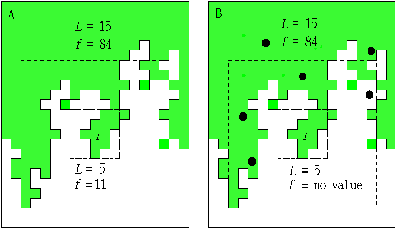
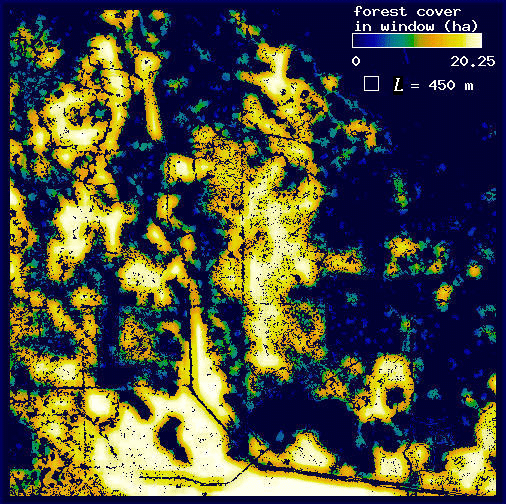
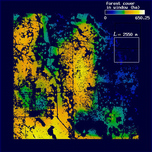
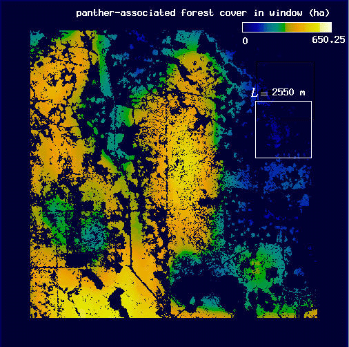
In order to estimate D for each plot, we followed Voss (1988) to measure the expected amount of forest F(L) for a variety of window widths L. Here, windows may be thought of as analogous to the square quadrats common in ecological research. In each plot, we centered a window of width L on each forest pixel and tallied the number of forest pixels found in the window. We then mapped the sum, f, as the value of the center pixel (Fig. 3 and Appendix). We calculated the expected number of pixels F(L) in a window of width L as the mean f over all of the forest pixels. Voss (1988) uses a more complicated probability density function calculation, but for our more restricted analysis, the mean is both sufficient and computationally simpler. We then incremented L and repeated the procedure to find F for each window width. Finally, we estimated D as the slope of a least squares regression of log F(L) on log L.

Fig. 3. (A) A schematic for the windowing procedure used to measure forest cover (green). A window of width L = 5 pixels is centered on a forest pixel and the number of forest pixels in the window f is mapped to the value of the center pixel. Once all forest pixels have been measured in this way, F(5) is calculated as the mean value of f over all forest pixels. At larger window sizes (e.g., L = 15 pixels), the procedure is repeated. (B) A contrasting schematic for the conditional mapping procedure. For L = 5, there are no panther locations (circles) in the window around the center pixel; hence, f receives no value, i.e., it is "not associated" with panther locations. After all forest pixels have been measured, H(5) is calculated as the mean of f only over those pixels found to be associated with panther locations. For L = 15 pixels, panther locations are found in the window and the f value of the center pixel is mapped for the calculation of H(15).

We began with a window width of 7 pixels (210 x 210 m) and proceeded in increments of 10 pixels (300 m) up to a maximum window width of 307 pixels (9210 x 9210 m). To eliminate edge effects, we used only data points whose largest corresponding windows fit fully within the extent of the plot. For clarity, we express F(L) in terms of forest cover area (hectares), rather than a pixel count. To do so, we simply multiply the count by the area of a single pixel (0.09 ha).

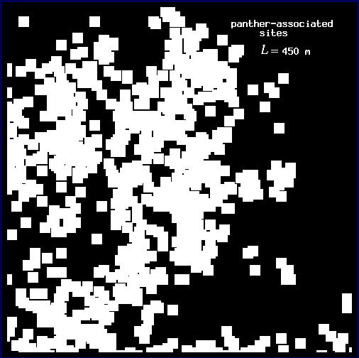
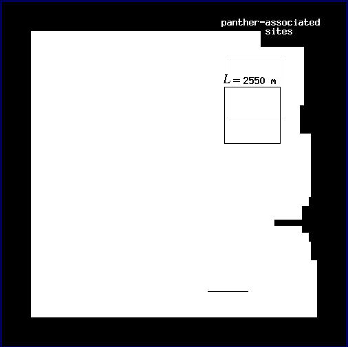
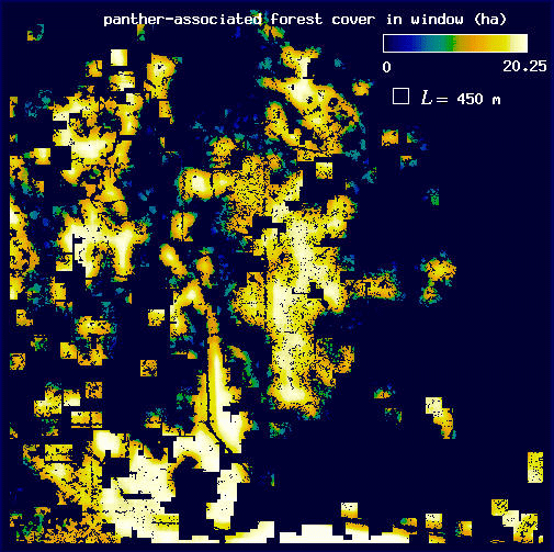
Conditional mapping

Forest areas used by panthers are likely to differ from typical forest areas in some measurable way, and the correlation between panthers and forest may vary with scale (see Milne et al. 1989). Association is a scale-dependent notion, and the spatial distribution of forest subsets associated with panther locations will change with the scale at which association is defined. To account for this scale dependence, we utilized a conditional mapping approach (Milne 1992, 1997, Scheuring and Riedi 1994; Appendix) to delineate the subset of forest associated with panther locations at different scales. Centering a window of width L on each forest pixel, we searched for panther locations within the window. If at least one panther location occurred in the window, the forest pixel was considered to be associated with panther locations at scale L. Otherwise (no panther locations in the window), it was considered non-associated (Fig. 3 and Appendix). The specific pixels associated with panther locations change as the window width L changes (see Appendix).

We then used a variation on the method described above to calculate H(L), the expected amount of panther-associated forest at scale L, for each plot. For each window width L, we again centered a window on each forest pixel and summed the number of forest pixels present in the window, mapping the sum f to the center pixel. Next, we eliminated those forest pixels that were not associated with panthers at scale L (i.e., those forest pixels whose windows contained no panther locations; Appendix). We then found H(L) by taking the mean value of f over the remaining forest pixels. It is important to note that as L increases, an ever greater proportion of the forest pixels is included in the calculation of H(L) because large windows are more likely to include a panther location (see Appendix). Thus, in the limit of very large L, all of the forest points are associated with panther locations and H(L) is expected to converge to F(L). Thus, the analysis is most sensitive to fine-scale habitat choices on the part of the panther.

Despite the fact that the spatial distribution of forest points associated with panthers is different for each window width L, H(L) may still vary systematically with L. If the distribution remains fractal, H(L) should follow a power law analogous to Eq. 2.

  (5)

Here, g is a proportionality constant and E is an exponent analogous to the fractal dimension D of Eq. 2. As before, we estimated E using a least squares regression of logH(L) on logL and looked for systematic deviations from power law scaling on log-log graphs of H(L) on L.

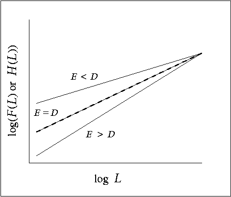
Assuming a good fit for the scaling relations (Eqs. 2 and 5), using a paired t test to compare the scaling exponents (E and D) gives us a way to assess the relationship between the forest at large and the subset associated with panther locations across scales. Given that H(L) must eventually converge to F(L) for large values of L, we defined three alternative possibilities (Fig. 4). (1) If E = D, forest points associated with panthers are a representative sample of the forest at all scales. (2) Alternatively, if E < D, panther-associated forest is denser than the forest at large at fine scales (small L), indicating panther preference for locally dense forest areas, as we hypothesized. (3) Conversely, E > D means that panther-associated forest is a sparser subset of forest for small L. The final alternative might be expected if panthers were routinely selecting forest edges, which are, by definition, sparser than patch interiors.

Fig. 4. Three alternative hypotheses relating the scaling behavior of forest associated with panthers, H(L), described by E (the slope of the solid lines), to that of the forest at large F(L), described by D (the slope of the dashed line). Prior to log transformation, y-axis values were measured in hectares and x-axis values in meters).

We calculated H(L) over the same range of L values as F(L) so that comparisons could also be made discretely for each value of L. A comparison of H(L) to F(L) is a comparison of forest density associated with panther locations to that of the available forest cover. For each window width L, we used a paired t test to determine whether panthers were selecting a locally dense subset of forest, i.e., whether H(L) > F(L) consistently across plots, corresponding to alternative (2) above. Because H(L) must converge to F(L), we expected that differences between H(L) and F(L) would be harder to detect as L increased.

As a caveat, this method makes no distinction between those forest points associated with one panther location and those associated with several. Thus, we are assuming that any forest point associated with even one panther location is in some sense "good habitat." Although weighting the contribution of each forest pixel to the mean H(L) by the density of panther locations associated with it may be a solution, the development and evaluation of such a technique lies beyond the scope of this work.

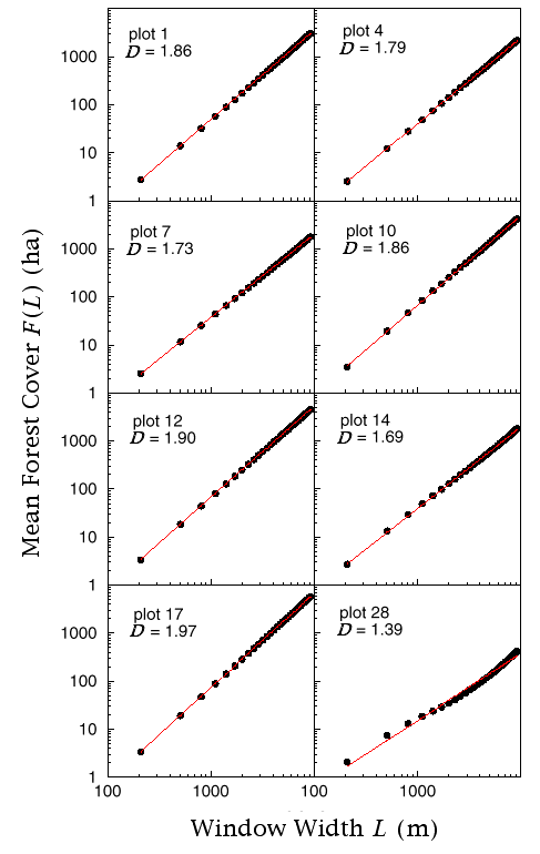
The power law scaling of forest cover was supported by its generally high degree of fit in all 28 forest plots (Fig. 5), indicating an overall fractal distribution of forest cover that could be characterized by Eq. 2, with values of D ranging between 1.22 (plot 27) and 1.97 (plots 17 and 22). Use of a fractal model to describe the forest was further validated by the strength of D as a predictor of percent cover assessed on the scale of the entire plot (Fig. 6; F = 132.34, df = 27, percent forest cover = 0.007e^(4.47D), r² = 0.84, P < = 0.0001), even though window widths used to estimate D were restricted to less than one-third of the plot width and measured only the center one-half of the plot.

Fig. 5. Scaling relations for the expected amount of forest F(L) for a random subset of study plots.

Fig. 6. Relationship between forest fractal dimension D and percent forest cover assessed at the scale of the plot, described by an exponential model.

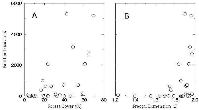
Neither percent cover nor D provided a clear predictor of panther locations (Fig. 7). Forest fractal dimension D, however, more strongly suggested a threshold phenomenon in the number of panther locations, with no extensive panther aggregations where D < = 1.8 (Fig. 7B). This threshold corresponds to approximately 25% forest cover at the scale of the entire plot (Fig. 6), but the clarity of the threshold is less pronounced if forest cover is measured at a single scale (i.e., Fig. 7A).

Fig. 7. Number of panther locations per plot as a function of (A) percent forest cover in plot, and (B) forest fractal dimension D.

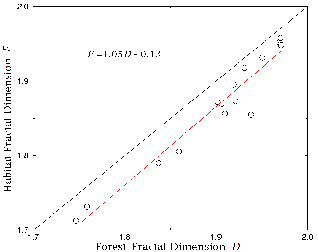
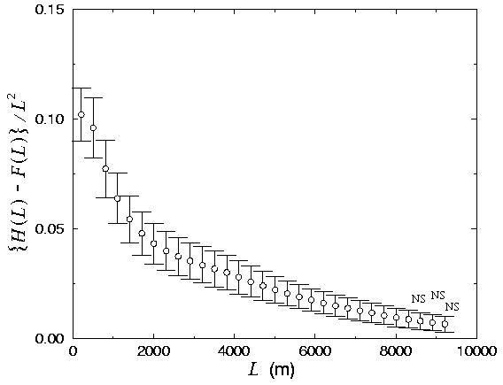
In the case of the conditional mapping analyses, all 15 plots exhibited a very high degree of fit to the scaling relation (Fig. 8). As predicted for the case of panthers selecting locally dense forest sites, H(L) values tended to be slightly higher than F(L) for small values of L (Fig. 8), with a consequent difference between the fractal dimensions D and E (paired t test, N = 15, t = -6.8, P = 0.0001), with E < D in every plot (Fig. 9). The difference between H(L) and F(L), expressed in terms of density (as in Eq. 4), was relatively small for any value of L (Fig. 10). However, these differences were statistically significant for all but the largest L values (Fig. 11).

Fig. 8. Scaling relations for the expected amount of forest associated with panther locations (H(L), shown as plus signs). Scaling relations for F(L), in circles, are included for comparison.

Fig. 9. Fractal dimension of forest associated with panthers, E, as a function of the fractal dimension of the forest at large D. The dotted line is 1:1.

Fig. 10. Density of forest (mean +/- 1 SE) associated with panthers (open circles) and the forest at large (solid squares) as a function of window width L. Mean and standard error are calculated over the 15 plots used in the conditional mapping analyses.

Fig. 11. Difference between density of the forest associated with panthers and the forest at large, as a function of scale. NS indicates no significant difference (paired t test; P > 0.05).

Forest fractal dimension D describes the expected increase in forest cover as panthers increase their search distance (Fig. 1). It provides an ecologically meaningful basis for explaining interactions between the panther and forest cover because it describes the marginal rate of gain in forest cover for an increase in search area. Areas of high D allow panthers to obtain ample resources (forest) for metabolic and reproductive maintenance within a relatively small search area, and permit relatively dense panther aggregations. Conversely, in areas with lower D, panthers have to expend more effort and range more widely to accumulate sufficient resources, and panther locations become necessarily sparser. In contrast, measurements of forest density made at a single, arbitrary scale necessarily fail to characterize gain in habitat as a function of increased effort. Single-scale measurements also provide no means of extrapolation to broader scales (as in Fig. 6), which is a critical concern in the conservation of the extensive ranges required by large animals.

Remarkably, the forests of South Florida maintained continuous fractal scaling even in the vicinity of intense human development (e.g., Fig. 2, plot 3). Anthropogenic disturbance may impose a characteristic scale on the landscape that disrupts the fractal scaling of vegetation cover. The absence of such an effect here indicates that the factors that maintain patterns of forested vegetation have not been completely overwhelmed (Krummel et al. 1987). A fractal characterization of the forest also makes the potential effect of continued anthropogenic habitat loss on the panther quite clear (Fig. 7B). When D drops below the threshold 1.8 (corresponding to about 25% forest cover on the scale of a plot; Fig. 6), the likelihood of intensive panther use declines dramatically. Similar nonlinear responses to fragmentation have been observed in the American marten (Bissonette et al. 1997). The study area as a whole exhibits about 22% forest cover, implying that the region may be, from a panther-centered view, on the verge of collapse. Although extrapolating the relationship in Fig. 6 to such broad regional scales introduces considerable uncertainty in the exact value of the threshold, the nature of the risk remains the same. Further loss and fragmentation of forests (pushing the region below the threshold, whatever its exact value may be) could cause drastic, nonlinear decreases in the panther population.

The fact that several plots exhibited D > 1.8 but contained few, if any, panther locations suggests that, above the threshold, panthers respond to other environmental influences in addition to forest cover. Below the threshold, these reponses are unimportant because there is simply too little resource to sustain resident panthers. Thus, the threshold may be thought of as a bifurcation point, with one state below the threshold ("no panthers") and two alternative states ("no panthers" or "panthers") above it, with the resulting state determined by a multitude of environmental factors as well as forest cover. In planning reintroduction (Jordan 1997), it will thus be important to consider other factors, such as water level and potential barriers to dispersal, only once the threshold fractal dimension (or density) of forest has been exceeded.

Where panthers do reside, they appear to select locally dense forest areas (Figs. 8 and 10). Selection seems strongest at fine scales (i.e., L = 200-1500 m; Fig. 11), implying that local forest density is of particular importance to panthers, an observation corroborated by Maehr (1997a). However, the fact that significant differences between H(L) and F(L) persisted even for scales in excess of L = 8 km indicates that panthers may be integrating spatial information concerning forest cover and selecting habitat over quite broad scales (a window of width L = 8310 m contains an area of 69 km², which is approximately two-thirds the average area of a female panther home range or about one-fifth that of a male; Maehr 1997a). This result is especially striking, considering that the method should be relatively insensitive to differences between H(L) and F(L) for large values of L. A more sensitive analysis might reveal selection at even broader scales. In some parts of the panther's range, the selection of especially dense areas at broad scales may be limited by the regional availability of large, unfragmented forest patches. This sort of broad-scale limitation may restrict the panther population to the central part of its range (e.g., Fig. 2, plots 9, 12, 17, and 21). The surrounding smaller patches (Fig. 1, plots 8 and 16) gain value as panther habitat due to their proximity to large, unfragmented forest tracts.

Taken as a whole, the conditional mapping results imply that panthers do indeed interact with forest cover at multiple scales (sensu Wiens 1989, Holling 1992). Thus, management of the existing panther population cannot focus on large forest patches alone. Depending on their broad-scale context, even small forest patches may be essential to the persistence of the population. In the next section, we attempt to develop a protocol for evaluating forest with respect to panthers at multiple scales. The protocol should not be considered a means of evaluating panther habitat per se. As we have noted, some threshold rate of forest gain, described by D, seems to be a necessary, but not sufficient, criterion for panther residence in an area. Instead, we hope to represent a view of the forest that is incrementally more panther-centered than a picture of the forest cover data alone.

Toward a panther-centered view

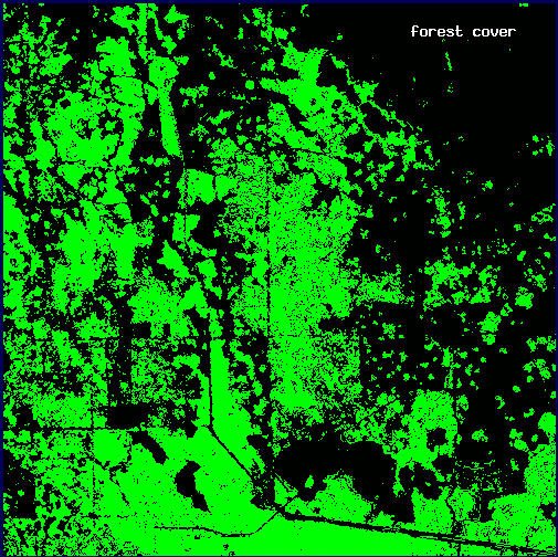
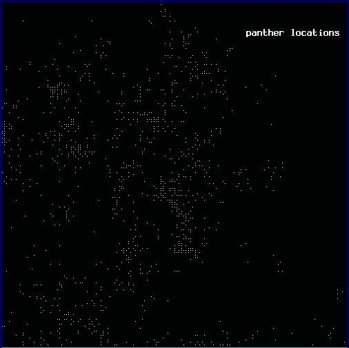
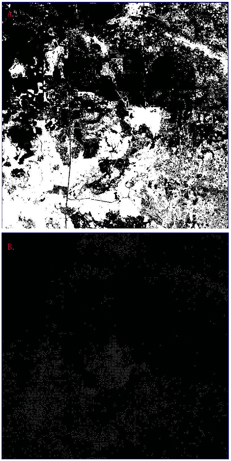
Working under the hypothesis that, for panthers, the most valuable forest areas are those that exhibit high density at multiple scales, we constructed a map of forest density at three scales. We selected plot 12 (see Fig. 2) as an example because it exhibits a high degree of heterogeniety in both forest cover (Fig. 12A) and its distribution of panther locations (Fig. 12B). Constructing the map is relatively simple. We first mapped forest density at each scale, then selectively eliminated forest points based on thresholds drawn from the previous analyses of panther association, and finally combined the three density maps into a single image.

Fig. 12. Sample plot used to construct a multiscale density map: (A) forest cover (white); (B) panther locations (white). (See plot 12, Fig. 2)

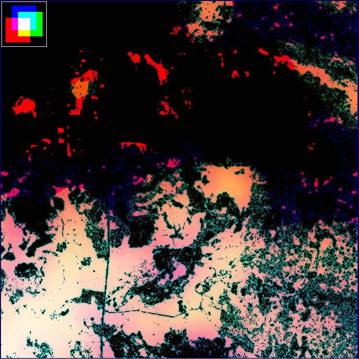
The first step was accomplished by repeating the windowing procedure described previously (see Methods and the Appendix). We selected window sizes of L = 210, 3210, and 8310 m. The extremes represent the minimum scale of our analysis and the maximum scale at which H(L) could be distinguished from F(L); the middle value is an arbitrary intermediate scale. Once window sums had been mapped, we converted them to density by dividing each pixel value by the area of the window L². For each resulting density map, we then established a threshold density using the mean density of forest associated with panthers for that value of L (mean H(L)/L² calculated over all 15 plots; Table 1, Fig. 10). For each map, if a forest pixel was more than two standard deviations below the threshold density, its value was set to 0 (nonforest). This procedure selectively eliminated forest pixels independently at each scale, based on a low likelihood of being associated with panthers (Fig. 13). To view the three maps together, we projected each with a different color band of the computer display. Red was used for fine-scale density, green for intermediate scale density, and blue for broad-scale density; brightness increased with density (Fig. 14).

Fig. 13. Forest cover mapped at three scales thresholded by the mean panther-associated forest density: (A) L = 210 m; (B) L = 3210 m; (C) L = 8310 m.

Fig. 14. Three forest density maps (Fig. 13) as a single image. Fine-scale density (L = 210 m) is mapped using red; the intermediate scale (L = 3210 m) using green; and broad-scale density (L = 8310 m) using blue. Brightness of each color increases with density at the corresponding scale. Colors combine as in the key at upper left, with variation due to the relative brightness of each color component.

Several observations can be drawn from a simple qualitative comparison of Fig. 14 to the original maps of forest and panther locations (Fig. 12). First, panther locations tend to be concentrated in white and pink areas, representing areas with relatively high density at all three scales (e.g., Fig. 14, southwestern corner). Second, the areas of forest eliminated by the thresholding procedure do not appear to be used extensively by panthers. Third, areas of high fine-scale density (bright red) seem to receive some panther use if they are near areas of multiscale density (white/pink). Finally, panther locations seem to decrease in density as areas of high density at all three scales become progressively fragmented (e.g., Fig. 14, southeastern corner).

We emphasize that all of these observations are purely qualitative and exceptions can be pointed out for each one. However, they do support our working hypothesis that panthers prefer forest areas that are dense at multiple scales. Further, our observations suggest that a protocol similar to ours, with testing and refinement, could be developed to aid in the estimation of currently available panther habitat and the evaluation of potential reintroduction sites, especially if other factors such as hydrology could be accounted for. In general, this sort of multiscale assessment could help to inform environmental management in a world that demands policy decisions at multiple scales in the face of high uncertainty (Walters 1997). Although the techniques are relatively new, advances in computing power and GIS technology have made them accessible to a wide spectrum of management agencies and environmental stakeholders. Further development in this area is ongoing (e.g., Bissonette 1997).

Panthers select densely forested habitat at multiple scales. The maintenance of forest cover is thus critical to the persistence of the subspecies. If citrus development, urbanization, or water flow regulation negatively impact the forests of South Florida, at any scale, the panther population will also be impacted detrimentally. Even at fine scales, further forest loss could cascade through the entire panther population, as individuals reorganize their home ranges to accommodate the human imposition. Local adjustments of this kind have been observed in breeding panthers (Maehr 1997b). Although the panther population may not be robust enough to endure manipulative tests of this hypothesis, the continued development of South Florida provides one large, irreversible experiment.

Responses to this article are invited. If accepted for publication, your response will be hyperlinked to the article. To submit a comment, follow this link. To read comments already accepted, follow this link.

We wish to thank the Florida Game and Freshwater Fish Commission for data collection. Financial support for A. J. Kerkhoff was provided by the NSF Graduate Research Traineeship in Ecological Complexity, Wilkison and Associates, Inc., the ATLSS project, and the University of New Mexico Department of Biology Graduate Research Allocations Committee. E. H. Decker, C. E. Restrepo, G. C. Stevens, G. Peterson, P. S. Bourgeron, B.-L. Li , C. S. Holling, G. Henebry, and four anonymous reviewers made helpful comments on earlier drafts.

Belden, R. C., W. B. Frankenberger, R. T. McBride, and S. T. Schwickert. 1988. Panther habitat use in southern Florida. Journal of Wildlife Management 52:660-663.

Bissonette, J. A., editor. 1997. Wildlife and landscape ecology. Springer-Verlag, New York, New York, USA.

Bissonette, J. A., D. J. Harrison, C. D. Hargis, and T. G. Chapin. 1997. The influence of spatial scale and scale-sensitive properties in habitat selection by American marten. Pages 368-385 in J. A. Bissonette, editor. Wildlife and landscape ecology. Springer-Verlag, New York, New York, USA.

Clark, J., J. Dunn, and K. Smith. 1993. A multivariate model of female black bear habitat usage for a geographic information system. Journal of Wildlife Management 57:519-526.

Cox, J., R. Kautz, M. MacLaughlin, and T. Gilbert. 1994. Closing the gaps in Florida's wildlife habitat conservation system. Office of Environmental Services, Florida Game and Fresh Water Fish Commission. Tallahassee, Florida, USA.

Delcourt, H. R., P. A. Delcourt, and T.Webb, III. 1982. Dynamic plant ecology: the spectrum of vegetational change in space and time. Quaternary Science Review 1:53-175.

Holling, C. S. 1992. Cross-scale morphology, geometry, and dynamics of scosystems. Ecological Monographs 62:447-502.

Jordan, D. B. 1997. Identification and evaluation of candidate Florida panther population reestablishment sites. Pages 106-152 in D. B. Jordan, editor. Proceedings of the Florida Panther Conference,1-3 November 1994, Ft. Myers, Florida, USA. U.S. Fish and Wildlife Service.

Kautz, R. S., D. T. Gilbert, and G. M. Mauldin. 1993. Vegetative cover in Florida based on 1985-1989 Landsat thematic mapper imagery. Florida Scientist 3:135-154.

Keitt, T. H., D. L. Urban, and B. T. Milne. 1997. Detecting critical scales in fragmented landscapes. [online] 1(1):4. URL: http://www.consecol.org/vol1/iss1/art4/

Krummel, J. R., R. H. Gardner, G. Sugihara, R. V. O'Neill, and P. R. Coleman. 1987. Landscape pattern in a disturbed environment. Oikos 48:321-324.

Levin, S. A. 1992. The problem of pattern and scale in ecology. Ecology 73:1942-1968.

Maehr, D. S. 1997a. The comparative ecology of bobcat, black bear, and Florida panther in South Florida. Bulletin of the Florida Museum of Natural History 40:1-176.

Maehr, D. S. 1997b. The Florida panther: life and death of a vanishing carnivore. Island Press, Covelo, California, USA.

Maehr, D. S., E. D. Land, and J. C. Roof. 1991. Social ecology of Florida panthers. National Geographic Research and Exploration 7:414-431.

Maehr, D. S., and J. A. Cox. 1995. Landscape features and panthers in Florida. Conservation Biology 9:1-13.

Mandelbrot, B. B. 1982. The fractal geometry of nature. W.H. Freeman, New York, New York, USA.

Meentemeyer, V. 1989. Geographical perspectives of space, time, and scale. Landscape Ecology 3:163-173.

Milne, B. T. 1991. Lessons from applying fractal models to landscape patterns. Pages 199-235 in M. G. Turner and R. H. Gardner, editors. Quantitative methods in landscape ecology. Springer-Verlag, New York, New York, USA.

Milne, B. T. 1992. Spatial aggregation and neutral models in fractal landscapes. American Naturalist 139:32-57.

Milne, B. T. 1997. Applications of fractal geometry in wildlife biology. Pages 32-69 in J. A. Bissonette, editor. Wildlife and landscape ecology. Springer-Verlag, New York, New York, USA.

Mladenoff, D. J., T. A. Sickley, R. G. Haight, and A. P. Wydeven. 1995. Regional landscape analysis and prediction of favorable gray wolf habitat in the northern great lakes region. Conservation Biology 9:279-294.

O'Neill, R. V., D. L. DeAngelis, J. B. Waide, and T. F. H. Allen. 1986. A hierarchical concept of ecosystems. Princeton University Press, Princeton, New Jersey, USA.

Scheuring, I., and R. H. Riedi. 1994. Application of multifractals to the analysis of vegetation pattern. Journal of Vegetation Science 5:489-495.

Senft, R. L., M. B. Coughenour, D. W. Bailey, L. R. Rittenhouse, O. E. Sala, and D. M.Swift. 1987. Large herbivore foraging and ecological hierarchies. BioScience 37:789-799.

Turner, M. G., and R. H. Gardner. 1991. Quantitative methods in landscape ecology: an introduction. Pages 3-14 in M. G. Turner and R. H. Gardner, editors. Quantitative methods in landscape ecology. Springer-Verlag, New York, New York, USA.

Urban, D. L., R. V. O'Neill, and H. H. Shugart. 1987. Landscape ecology. BioScience 37:119-127.

Voss, R. F. 1988. Fractals in nature: from characterization to simulation. Pages 21-70 in H. O. Peitgen and D. Saupe, editors. The science of fractal images. Springer-Verlag, New York, New York, USA.

Walters, C. J. 1997. Adaptive policy design: thinking at larger spatial scales. Pages 386-395 in J. A. Bissonette, editor. Wildlife and landscape ecology. Springer-Verlag, New York, New York, USA.

Wiens, J. A. 1989. Spatial scaling in ecology. Functional Ecology 3:385-397.