Scientist: The scientist (Monitoring, Assessment and Forecasting component of Carpenter et al. 1999) measures the phosphorus load to the system and the current water phosphorus levels, and makes these data available to the economist. The scientist also fits a forecasting model to predict the response of P levels in the lake to future inputs (Appendix 3 of Carpenter et al. 1999). This fitting process yields a reversibility parameter, which provides an index of the capacity of the lake to withstand increases in P input (Appendix 2 of Carpenter et al. 1999).

Economist: The economist receives data from the scientist and generates two sets of loading recommendations - one based on free information and the other based on costly information (Appendix 3 of Carpenter et al. 1999). In addition, the economist evaluates the economic impact of the most recent phosphorus load.

Agents: Agents review past performances of free and costly policies and decide whether or not to buy the costly loading recommendation. The final target phosphorus load is the aggregate of all individual agent choices.

Ecosystem: Once the agents set a target phosphorus load, nature introduces a random load disturbance that adjusts the target either up or down. Once the phosphorus load enters the lake, the lake responds with its intrinsic phosphorus cycling mechanisms (Appendix 1 of Carpenter et al. 1999).

You the game player: You control the cost of the information and the intensity parameter (chi in Appendix 4 of Carpenter et al. 1999). The intensity parameter controls the magnitude of an agent's response to a given difference in expected performance between the costly and free information.

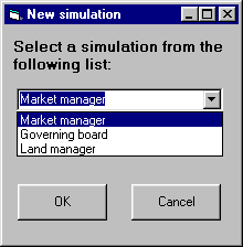
To create a simulation, simply follow these four steps.

The simulation specific controls allow you to play a role in the simulation. In this simulation, your role as the information market manager allows you to change the information cost and the preference intensity. Both of these parameters affect the agents’ decisions when choosing free or costly information.

Information Cost: As you might guess, this control adjusts the price that agents pay for information when they choose to buy information. The range is from 0.01 to 2.0. When the Mark box is checked, changes you make to the slide bar show as white triangles in the graphs at the following x,y coordinates: x = year, y = proportion of maximum possible information cost. You can adjust the slide bar at any time during the simulation.

Preference Intensity: Changing preference intensity adjusts the chi parameter in the agents’ choice equation,

where N is the proportion of agents choosing action i, and Vi is the value expected under action i (see: Appendix 4: Management via Information Market in the manuscript for details). The intensity parameter controls the magnitude of an agent's response to a given difference in expected performance between the costly and free information. The range of this control is from 10 to 1,000. When the Mark box is checked, changes you make to the slide bar show as red triangles in the graphs at the following x,y coordinates: x = year, y = proportion of maximum possible preference intensity. You can adjust the slide bar at any time during the simulation.

All output graphs run synchronously, with years being the x axis unit. All line data are plotted on the left y axis. The white and red marks are plotted on the right y axis, with the scale, ranging from zero to one, representing the proportion of maximum for the given simulation specific control.

Graph 1: Target Phosphorus and Actual Phosphorus Loads

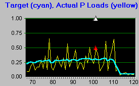
Scientists provide data about their perception of the ecological system to economists, who in turn provide either free or costly phosphorus loading recommendations to the agents. The target load represents the aggregate targets of the two agent types. Actual loads vary around the targets due to unpredictable loading phenomena, such as changes in weather. The simulation introduces stochasticity in the phosphorus load calculation.

The white and red marks indicate that the user changed information cost and preference intensity, respectively, on year 100. Information cost was set to its maximum of two; whereas, preference intensity was set to half its maximum of 1,000.

 Graph 2: Water Phosphorus and Net Payoff

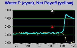
Water phosphorus remains relatively low (<0.3) until an unusually high random phosphorus load on year 110 (see graph 1) helps kick it into its alternate stable state. This consistently high phosphorus level indicates that the lake has turned eutrophic, and its economic value suffers. Net payoff (units are adjusted to fit the y axis) takes a plunge, but begins recovery as the lake phosphorus drops from year 110 to 120 and beyond.

Notice the proximity of the white and red markers to the flip. The relationship between parameter changes and lake-state are subject to your interpretation.

Graph 3: Reversibility Parameter

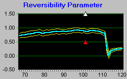
The reversibility parameter represents the scientist's belief that the system can recover quickly from perturbation. A value less than about 0.5 means that the scientist believes that a large influx of phosphorus to the lake could cause irreversible damage. As the values rise, the scientist's confidence that the lake could recover from a sudden influx of P rises. Keep in mind that the scientist does not know the true reversibility, but is merely estimating it.

 

 

Graph 4: Agents Using Free Information vs. Agents Buying Information

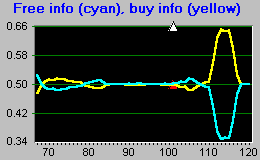
Agent proportions change as their interpretations of past events and their predictions for the future change, and as the cost of information changes. On year 100, the user set the information cost to its maximum, which seemed to trigger a period of freeloading.

Freeloading quickly gave way to buying as the lake flipped states. By about year 120 the proportion of agents buying information returned to its typical value of about 0.5.

NonPoint measures your performance by calculating the percentage of days when lake phosphorus was less than one, and by calculating your cumulative payoff (values adjusted to match the scale). These measures help you to determine relative performance between simulations.

NonPoint displays the overall mean percentage of agents using free information and agents buying information. Thus far in the simulation the buyers and freeloaders are near evenly split, with the buyers maintaining a slight advantage.