|
|
|
Copyright © 1997 by the Ecological Society of America
Keitt, T.H., D.L. Urban, and B.T. Milne. 1997. Detecting critical scales in fragmented landscapes. Conservation Ecology [online]1(1): 4. Available from the Internet. URL: http://www.consecol.org/vol1/iss1/art4/
A version of this article in which text, figures, tables, and appendices are separate files may be found by following this link.
Research
Detecting Critical Scales in Fragmented Landscapes
Timothy H. Keitt1, 2 Dean L. Urban3 Bruce T. Milne1
1Department of Biology, University of New Mexico; 2Santa Fe Institute; 3School of the Environment, Levine Science Research Center, Duke University
We develop methods for quantifying habitat connectivity at multiple scales and assigning conservation priority to habitat patches based on their contribution to connectivity. By representing the habitat mosaic as a mathematical "graph," we show that percolation theory can be used to quantify connectivity at multiple scales from empirical landscape data. Our results indicate that connectivity of landscapes is highly scale dependent, exhibiting a marked transition at a characteristic distance and varying significantly for organisms with different dispersal behavior. More importantly, we show that the sensitivity and importance of landscape pattern is also scale dependent, peaking at scales associated with the percolation transition. In addition, the sensitivity analysis allows us to identify critical "stepping stone" patches that, when removed from the landscape, cause large changes in connectivity.
KEY WORDS: connectivity, conservation in fragmented landscapes, dispersal, fragmentation, habitat connectivity vs. dispersal distance, landscape, landscape graphs, metapopulation, percolation, quantifying habitat connectivity at multiple scales, "stepping stone" patch, Strix occidentalis lucida.
Connectivity of landscapes depends not only on the spatial distribution of habitats across a landscape, but also on the scale at which organisms interact with landscape pattern (Merriam 1984, Gardner et al. 1989, Noss 1991). In fragmented landscapes, where islands of high-quality habitat are punctuated by stretches of poor habitats, species that disperse over long distances will perceive a given habitat distribution as more connected than will a species with short-range dispersal. Thus, landscape pattern can act as a scale-dependent "filter" acting differentially on the movement of species with different degrees of vagility, in much the same way as high- and low-pass filters remove high and low frequency components in a communication channel (Shannon and Weaver 1949). In relatively continuous landscape mosaics, where habitat quality varies smoothly, it is likely that the filtering effect of landscape pattern will also be smooth, reducing the rate of movement of some species while enhancing that of others (Johnson et al. 1992a, b). In highly fragmented landscapes, the filter response might be much more abrupt: species that perceive the habitat distribution below a critical scale could be effectively isolated on individual habitat patches. Therefore, particularly in fragmented landscapes, identification of critical scales associated with abrupt changes in landscape connectivity is an important consideration in quantifying habitat pattern and the influence of habitat pattern on the movement of organisms.
Landscape connectivity does not depend on scale alone; the configuration or spatial arrangement of habitats in a landscape is also an important determinant of connectivity (Forman and Baudry 1984, Gardner et al. 1992, Henein and Merriam 1990, Taylor et al. 1993). Heterogeneity in habitat quality, differences in patch shape and size, and variation in isolation among patches lead to spatial variation in landscape connectivity (Gustafson and Gardner 1996). Thus, although indices of landscape connectivity averaged over entire landscapes are useful for comparisons among ecosystems, these indices provide little insight into the local connectivity structure of landscapes. To fully characterize the spatial structure of landscapes, it is necessary to consider connectivity measures associated with local regions or individual habitat patches. Just as overall measures of landscape connectivity are scale dependent, local measures of connectivity are likely to change with scale.
Here, we present a multiscale analysis of landscape connectivity, based on an extension of uniform percolation theory (Stauffer and Aharony 1985, Gardner et al. 1987, Gould and Tobochnik 1988, Creswick et al. 1992) to non-uniform landscape graphs (Cantwell and Forman 1993, Harary 1969). We develop both aggregate measures of landscape connectivity and patch-based measures of individual patch contributions to overall connectivity. We examine the sensitivity of landscape connectivity to changes in landscape configuration, and the relationship between sensitivity and scale. Finally, we consider the implications of our analysis for habitat preservation efforts with regard to threatened species.
Landscape data
Our study site consisted of a 1.5 x 10⁶ km2 region of the southwestern United States, including the states of Arizona, Colorado, New Mexico, and Utah. The Southwest physiographic region is largely comprised of desert, rocky canyons, semiarid grassland, and piñon-juniper woodland, interspersed with numerous mountain ranges supporting both conifer and deciduous hardwood forests (McLaughlin 1986). From a digital cover map of the Southwest (Evans et al. 1993, Evans and Zhu 1993), we selected two forest cover types, mixed-conifer and ponderosa pine, to represent the habitat pattern of interest; all other cover types were considered "nonhabitat." The mixed-conifer habitat type was principally composed of Douglas-fir (Pseudotsuga menzesii ), white fir (Abies concolor ), and several species of pine (Pinus ponderosa, P. contorta ). The ponderosa pine habitat type was dominated by ponderosa pine (P. ponderosa ), but probably included some pine-oak woodlands as well. The habitat map had a grid-cell resolution of 1 km x 1 km.
Our original motivation for choosing ponderosa pine and mixed-conifer forest types was to approximate the distribution of suitable nesting habitat for Mexican Spotted Owls (Strix occidentalis lucida) within the southwestern United States. The data were used in developing a recovery plan for the Mexican Spotted Owl (Keitt et al.1995, USDI Fish and Wildlife Service 1995).
Landscape graphs
Because our study concerned the spatial relationships among landscape patches, we chose to represent the habitat distribution as a mathematical "graph" (Harary 1969). Graphs are composed of sets of points ("vertices") and lines ("edges") connecting vertices. Previous work has shown graphs to be a useful representation of landscape structures (Cantwell and Forman 1993), but have relied on purely subjective assignment of vertices and edges to landscape features.
We developed an objective means of generating landscape graphs (Fig. 1 ). The input data consisted of a raster habitat map with each grid cell assigned the value one if that cell corresponded to the chosen habitat type, and zero if the cell was considered nonhabitat. A patch was defined as a spatially contiguous set of habitat cells. Two habitat cells were considered to be in the same habitat patch if they were adjacent in the four cardinal directions or diagonally (northeast, northwest, and so on). Once the habitat patches were labeled, we assigned a graph vertex to each patch. Edges were placed between vertices if their corresponding patches were connected according to the criteria to be described. Thus, the landscape graph consisted of a set of vertices, one for each habitat patch, and a set of edges indicating connections among patches. For display purposes, vertices were placed at the geometric center of each patch.
FIG. 1. Construction of a landscape graph. This example landscape contains three separate habitat patches and a single habitat cluster, or ``subgraph.'' The three patches belong to a single cluster because there exists a path along the graph edges (solid lines) that connects all three patches. If either one of the edges shown were removed, there would be two habitat clusters. If all edges were removed, then there would be three habitat clusters, each consisting of a single patch.

Our initial labeling of the forest data produced > 6000 individual habitat patches, some as small as a single grid cell. We were concerned that the smallest patches might not represent true habitat patches, but rather noise introduced by classification errors. Thus, we developed a novel method of filtering potential classification errors from the data. Our approach was based on applying neutral models (Gardner et al. 1987) to divide patches into two groups: those that were likely to result from random error and those that were more likely to represent true habitat patches.
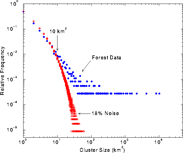
In classified landscape data, small habitat patches are much more likely to be the product of random error than are large patches. For example, if errors are introduced into an image with probability p << 1, then the probability of creating a patch of errors of size n is approximately p n. Random errors are unlikely to produce large patches, because as n increases, pn becomes very small. The forest data covered ~ 38% of the map area. Of the patches identified in the forest data, roughly 50% were single-cell patches. We calculated that a random map with 18% cover would also have 50% single-cell patches. Thus, an 18% error rate was sufficient to account for all single-cell patches (i.e., those most likely to be the result of classification error) in the forest data.
We then asked, over what patch sizes was the frequency of forest patches similar to the expected frequency of patches created by random noise? We plotted the frequencies of forest patch sizes and of patch sizes observed in 100 random maps with 18% density (Fig. 2 ), and found that the two distributions were similar up to a patch size of 10 km2 . Forest patches > 10 km2 in size occurred at much higher frequencies than patches of equivalent size in the random maps. Thus, we retained only patches >10 km2 in subsequent analyses.
FIG. 2. Relative frequency of patch sizes for Southwest forest data and for 100 random maps with density of 18%. Patch frequencies decay rapidly with increasing patch size for the random maps, but more slowly for the forest data. Forest patches >10 km2 in size occurred with much higher frequency than in the random maps, and were thus unlikely to have resulted from classification error.
Scaling analysis
In order to explore the effect of scale on landscape connectivity, we defined a patch connection criterion based on minimum distances between patches. We reasoned that the major barrier to dispersal would be gaps in habitat distribution across which an animal would have to travel to reach a neighboring patch. The extent to which these barriers limit animal movements and, hence, connectivity will, of course, depend on the scale at which an organism perceives landscape pattern. Species capable of long-distance dispersal will be less impacted by gaps in habitat distribution than will species with short-range dispersal. To emulate the effect of dispersal behavior on landscape connectivity, we constructed landscape graphs by placing edges between patches only if the minimum distance between them was less than a specified threshold. Sets of patches joined by edges formed "subgraphs" or isolated components of the graph. By varying the distance threshold, we were able to resolve the connectivity structure of the landscape across a wide range of scales.
Connectivity measures
Percolation theory is the study of connectivity in stochastically generated structures (Stauffer and Aharony 1985). Thus, connectivity measures developed in percolation theory were a natural choice as measures of landscape connectivity. Most applications of percolation theory in ecology (Gardner et al.1987) are based on lattice percolation, in which cells on a lattice are occupied with probability p and are left unoccupied with probability 1 - p. A standard mathematical result in lattice percolation is the emergence of a large "spanning cluster" at a critical probability pcrit. If connections between adjacent, occupied lattice cells are restricted to occur only in north, south, east, and west directions, then the critical probability is equal to 0.5928 (Stauffer and Aharony 1985). Other critical probabilities can be obtained by changing the connectivity rule, for example, by allowing connections to run diagonally (northeast, southwest, etc.) between occupied cells.
Percolation need not occur on a regular lattice. A more general model involves percolation on graph structures, referred to as "bond percolation" (Stauffer and Aharony 1985). Because regular lattices are a subset of possible graph configurations (Harary 1969), bond percolation naturally incorporates lattice percolation as a special case. In bond percolation, sites are either connected with probability p or are unconnected with probability 1 - p. As in lattice percolation, a large cluster of connected sites occurs at a critical value of p. Our application of percolation theory represents an extension of standard bond percolation. In our model, the probability of a connection between two habitat patches depends on the distance between the patches. Thus, the emergence of a spanning habitat cluster occurs at a critical mean dispersal distance instead of at a particular habitat density, as in traditional lattice percolation. Percolation problems where connection probabilities vary across the landscape are referred to as"gradient" or "non-uniform" percolation (Milne et al. 1996).
In percolation theory, connectivity is associated with the average size of connected clusters. A natural measure of the size of a circular cluster is its radius. However, in general, clusters are not round; they can be irregular, sinuous structures. Therefore, a measure of cluster size must control for irregular shapes. A measure of cluster size used in percolation theory is the "radius of gyration," defined as

where < x > and < y > are the mean x and y coordinates of lattice cells in the cluster, xi and yi are the coordinates of the ith grid cell in the cluster, and n is the total number of cells in the cluster (Creswick et al. 1992). Habitat clusters were defined as sets of patches connected by a subgraph or component of the thresholded landscape graphs. For a cluster comprised of several habitat patches, the sum in Eq. 1 was taken over all habitat cells among all patches in the cluster.
Unlike unitless indices of landscape connectivity, the cluster radius has units of distance and a direct physical interpretation. Imagine a randomly moving particle placed randomly on a habitat cluster. The radius of gyration is the average distance that the particle will move before encountering the cluster edge. Similarly, if a dispersing animal is restricted to moving on a particular habitat cluster (i.e., it has a low probability of traversing any gap separating it from another cluster), its average dispersal range will correspond to the radius of the cluster.
The size-weighted average connectivity of a set of clusters defines the correlation length of a landscape. The correlation length of a set of clusters is given by

where m is the number of clusters and ns is the number of grid cells in cluster s (Creswick et al. 1992). We used the correlation length as an overall measure of habitat connectivity in a landscape. As with the radius of gyration, correlation length has units of distance: it is the average distance an individual is capable of dispersing before reaching a barrier, if placed randomly on the landscape. Thus, as the correlation length increases, landscape connectivity increases.
Patch removal experiments
We wanted not only a measure of overall landscape connectivity, but also local measures of patch connectivity. In particular, we wanted to know the effect on landscape connectivity of removing a patch from the landscape. We designed a simple analysis in which each habitat patch was individually removed from the landscape. We recorded the change in the correlation length induced by removing each patch. Because the effect of removing a patch depended on scale, we repeated the patch removal analysis for a large number of distance thresholds. After a patch was removed, a new landscape graph was constructed. The connected subgraphs were then identified and the new correlation length was recorded. Letting C ( d ) be the correlation length of the landscape graph, thresholded at distance d , and C ( d, i ) be the correlation length after patch i was removed, then

is the normalized importance index of patch i. The normalized importance is a relative index of the contribution of each patch to overall landscape connectivity. We chose a normalized, unitless index because it was designed precisely for among-patch comparisons.
We expected that large patches would have larger importance indices, simply owing to their size. Thus, we wanted a measure of per area importance as well. The per area importance index quantified a patch's contribution to overall landscape connectivity per unit area. We defined the per area index as

where n ( i ) is the number of habitat cells in patch i and ac is the area of a grid cell. The per area index had units of 1/area, e.g., km-2.
Stochastic landscape graphs
To make percolation on landscape graphs equivalent to a bond percolation problem, it was necessary to define a stochastic function determining connections among patches. Because successful dispersal across gaps in the habitat distribution implies moving a distance at least, if not greater than, the minimum distance between patches, we used a cumulative probability distribution to indicate whether two patches were effectively connected for a given dispersal distance. For thresholded landscape graphs, the dispersal function was simply the step function

where d was the minimum distance between patches. An important property of the threshold function was that a given threshold distance resulted in only a single landscape graph structure. However, the percolation problem can be generalized to include any probability function. Beyond the threshold function, the simplest probability function is the cumulative negative exponential

where p ( d ) is the probability of dispersing at least distance d, and k is the dispersal coefficient. The dispersal coefficient has units of 1/distance; its inverse, 1/k, is the average dispersal distance under the distribution. Distributions requiring more parameters, such as the gamma distribution, could be used as well.
Unlike the threshold function, the negative exponential function resulted in a large number of landscape graphs for any given dispersal coefficient. Following standard techniques in percolation theory, we used a Monte Carlo procedure to generate multiple landscape configurations. We varied the dispersal coefficient, k , from 1.0 (average dispersal distance = 1 km) to 0.01 (average dispersal distance = 100 km). For each value of the dispersal coefficient, 100 randomly connected landscape configurations were generated and their correlation length was recorded. Connections between patches in each configuration were determined by comparing a uniform random number between 0.0. and 1.0 to the probability of dispersal occurring between patches, according to Eq. 6. If the random number was less than the the dispersal probability, the patches were joined into the same subgraph or cluster. Over many random configurations, the expected frequency of two patches being joined was equal to the probability of successful dispersal between them. Patches far apart were rarely connected, whereas patches whose borders were in close proximity were often connected, the frequency being determined by the dispersal coefficient.
Thresholded landscape graphs
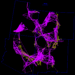
As the maximum interpatch dispersal distance was increased, the forest cover map became increasingly connected and eventually coalesced into a single, large graph spanning the entire habitat distribution (Fig. 3 ). At a 20-km threshold distance, the landscape was largely composed of independent patches and small habitat clusters. For organisms capable of dispersing 20 km, the landscape was highly fragmented. At 40 km, larger subgraphs formed, but the landscape was still divided into several habitat clusters. Above 40 km, most of the habitat distribution was connected. Although most of the habitat was joined at 50 km, only a single edge existed between the large subgraphs in the northeast and southwest of the habitat distribution. The vertices at either end of the single connecting edge are known as "articulation points," because removing either one would bisect the graph (Harary 1969). At a threshold distance of 80 km, the graph was highly interconnected and, in general, there were many alternate pathways from any one patch to another.
FIG. 3. Thresholded landscape graphs. An edge drawn between two habitat patches indicates a minimum distance between the patches less than or equal to the given threshold distance.
Click on each image to view in more detail. Please note that the detailed images are very large.
10 km 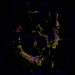 20 km
20 km 
30 km 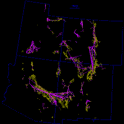 40 km
40 km 
50 km 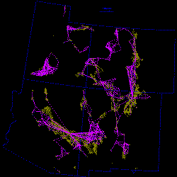 60 km
60 km 
70 km 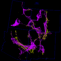 80 km
80 km 
90 km  100 km
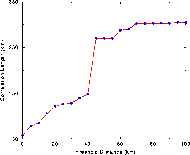
The sudden transition from a relatively disconnected distribution of habitat to a largely connected map appeared as an inflection in the plot of correlation length vs. threshold distance (Fig. 4 ). Between 40 and 45 km, the correlation length of the landscape nearly doubled, increasing from 150 km to ~275 km. A sudden change in connectivity at a critical density, or in this case a threshold distance, is referred to in percolation theory as a geometric "phase transition" (Stauffer and Aharony 1985). Thus, the landscape of habitat patches was divided into two separate"phases:"a connected phase and a disconnected phase.
FIG. 4. Correlation length of the habitat distribution vs. threshold distance.
Landscape sensitivity
The inflection in the correlation length not only separated the connected and disconnected phases of the map, but also was related to the landscape's sensitivity to habitat alterations. When patches were removed from the map, the effect on connectivity was highly scale dependent (Fig. 5 ). At short threshold distances, the effect of removing a patch was largely determined by its size, although shape also may have been important. At a 0-km threshold distance (all patches independent), the graph sensitivity was dominated by the largest patch.
FIG. 5. Graph sensitivity at different threshold distances. Patches are ordered by size. Sensitivity is the change in correlation length when a patch was removed.
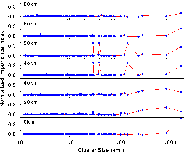
At longer threshold distances (30 and 40 km), several of the largest patches caused large deviations in the correlation length when removed. At 30- and 40 -km dispersal distances, the second and third largest patches composed the bulk of the graph. Up to this point (0-40 km), graph sensitivity was dominated by the largest patches. Thus, the relative position and orientation of patches mattered little: patch size was the most important factor determining importance.
The pattern of landscape sensitivity changed abruptly at 45 and 50 km. Although the largest patch still had a relatively high importance index, graph sensitivity (Fig. 5 ) exhibited several large spikes generated by much smaller patches. The large sensitivity associated with these patches was not due to their size; rather it reflected their role as "stepping stone" patches connecting large areas of habitat. These stepping stone patches corresponded to articulation points in the graph.
At distances above the transition (60 and 80 km), graph sensitivity returned to a pattern in which the largest patches were most important. However, the overall sensitivity was much lower, particularly at 80 km, because as the threshold distance was increased, the number of alternate pathways between any two patches increased, and the removal of any one patch had little effect on connectivity.
Patch importance
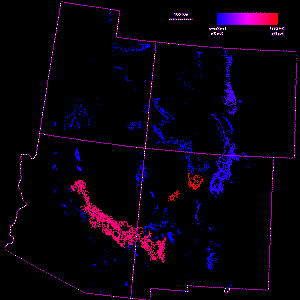
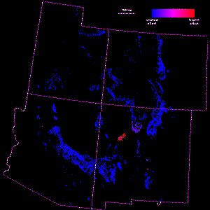
The contribution of individual patches to landscape connectivity was measured by removing each patch and recording the change in correlation length. Because the connectivity of the landscape was most sensitive to patch removal at scales near the percolation transition, we first analyzed the landscape at a threshold distance of 45 km (Fig. 6 ). As expected, the largest patch had the greatest contribution to connectivity. However, when weighted by area, a number of small patches also had large (per area) contributions to connectivity. These patches correspond to stepping stone patches connecting larger areas of habitat.
FIG. 6. Patch connectivity importance measures at 45-km threshold distance. [left: I (45 km, i ); right: A (45 km,i )].
Click on each image to view in more detail. Please note that the detailed images are very large.
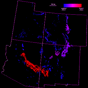
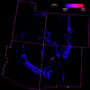
Because there is often uncertainty about which scale is most appropriate for analyzing connectivity, an average connectivity over a range of scales provides a more robust indication of patch importance. Patch importance values averaged over threshold distances from 0 to 100 km, in 5-km increments (Fig. 7 ), resulted in a pattern similar to that found at a 45-km threshold distance. However, the averaged importance index included a broader range of patches, corresponding to local percolation transitions at scales other than 45 km.
FIG. 7. Patch connectivity importance measures averaged over threshold distances from 0 km to 100 km. [left: I (0 -100 km, i ); right: A (0 -100 km, i )].
Click on each image to view in more detail. Please note that the detailed images are very large.
Connectivity in stochastic landscape graphs
Although the assumption of a maximum dispersal distance is useful for characterizing the connectivity of landscapes at different scales, it does not consider the stochastic nature of dispersal events. Therefore, we employed a Monte Carlo analysis, based on a dispersal probability function, to characterize the range of connectivities observed for different dispersal coefficients (see Eq. 6).
When the dispersal coefficient was varied between k =0.01 (i.e., long-range dispersal) and k =1.0 (i.e., short-range dispersal), the relationship between dispersal behavior and connectivity of the landscape was profoundly nonlinear, exhibiting a strong inflection at intermediate values (Fig. 8 ). Furthermore, the distribution of correlation lengths was clearly divided into two distinct phases, higher values indicating the connected phase and lower values the disjoint phase. At intermediate values, both phases existed for the same value of the dispersal coefficient. Thus, the phase transition observed previously for maximum dispersal distances was, in the Monte Carlo analysis, directly related to a particular dispersal coefficient. For forest habitats in the Southwest, the critical dispersal coefficient ( k c ) was ~ 0.06-0.07, i.e., an average dispersal distance of 14-17 km.
FIG. 8. Landscape connectivity for different dispersal coefficients. The coefficient is k in p(d) =e-kd where p(d) is the probability of an individual dispersing at least distance d . Each circle represents a single random landscape configuration.
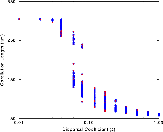
The range of connectivities for a given dispersal coefficient also exhibited marked differences as dispersal distances were increased. At either end of the plot (k =0.01 and k =1.0), the range of connectivity values was minimal. Long-range dispersal resulted in the landscape being connected for every Monte Carlo iteration. For short-range dispersal, the landscape was always fragmented. At intermediate dispersal coefficients, near the percolation transition, the range of connectivity values was much greater. The large range of connectivity values was again a reflection of the increased sensitivity found near a phase transition.
Our results clearly demonstrate that landscape connectivity is highly scale dependent. However, connectivity does not increase gradually with increasing scale. Instead, connectivity changes abruptly as the landscape undergoes a percolation transition. For the forest habitat distribution considered here, the transition occurred at a threshold distance of 45 km (Fig. 4 ), or, in the case of exponential dispersal probabilities, an average dispersal distance of ~ 15 km (Fig. 8 ). Thus, for an organism to perceive the habitat distribution as a single, large, interconnected cluster, it must, in general, be capable of dispersing a distance of 45 km over inhospitable habitat and must have an average exponential dispersal distance of at least 15 km.
An important finding of our analysis was that habitat loss has a highly scale-dependent effect on landscape connectivity. For organisms that perceive the landscape at fine scales, landscape configuration and stepping stone patches are of little consequence, because populations are restricted to local habitat patches. Similarly, movements of species capable of long-range dispersal will not be strongly influenced by the configuration of individual patches. For species near the percolation transition, landscape configuration may play a significant role in determining landscape connectivity. Near the percolation transition, individual patches can act as corridors or stepping stones, bridging gaps in the habitat distribution. Thus, we expect that landscape configuration will be important to species whose dispersal behavior places them near the landscape percolation threshold.
How applicable these results are to different species will depend to some extent on the mode of dispersal used. We designed our analyses to capture the essential features of owls dispersing between the "sky-island" habitats characteristic of the Southwest. Species using other modes of dispersal will interact with landscape patterns in a different manor. An organism that must walk or run over a landscape may encounter barriers not represented in our habitat maps. However, we see no reason why our approach could not be modified to incorporate other modes of dispersal and more detailed spatial information.
In general, we have too few data available to precisely predict dispersal patterns of Mexican Spotted Owls. However, there are several reports (reviewed in Keitt et al. 1995) of juvenile owls dispersing > 45 km, and it is typical, at least in some parts of the owls' range, for juveniles to establish new territories 10-20 km from their natal territory (Keitt et al. 1995). Thus, we believe that the Mexican Spotted Owls probably exist as a metapopulation and that landscape connectivity is an important consideration for their survival.
Management perspectives
Application of regional-scale habitat analyses to conservation ecology represents an important step forward, because it places management decisions within the landscape context and thus avoids local policies that fail to recognize critical linkages among populations. In particular, we believe that patch importance indices (Figs. 6 and 7) may prove useful in guiding habitat preservation efforts and designation of critical habitats, as well as the design of dispersal and demographic studies. For example, in our study of the Mexican Spotted Owl, one habitat area, the Mount Taylor ranger district in central New Mexico, had high importance indices across all analyses. The Mount Taylor region previously was not considered important habitat, because it contains relatively few owls. However, our analysis highlighted Mount Taylor as a stepping stone linking owl populations in southern New Mexico and Arizona to populations in Colorado and Utah. These northerly populations may exist as demographic sinks (Pulliam 1988), but nonetheless could act as buffers against collapse of source populations caused by disturbance or disease (Thomas et al. 1996).
The importance of regional- and landscape-scale analyses is even greater in situations in which multiple agencies manage habitats throughout a species range. For example, market forces may induce forest managers to harvest timber from a small region of habitat such as Mount Taylor, thinking that the patch is of little ecological importance. However, a high per area index (Fig. 6 ) for the same patch might lead managers to recognize the role of the patch as a crucial link within a broader region composed of several management jurisdictions. Alteration of the patch based on nonspatial, economic perspectives could jeopardize conservation goals among many agencies. Within a jurisdiction, such as a national forest, managers might reallocate harvests to patches that have small per area indices in order to preserve the connectivity value of the entire habitat network. Alternatively, one or more agencies may trade land or extracted resources to accomplish management goals while maintaining network fidelity.
We also wish to emphasize that our results are not restricted to single-species studies. Habitat patches that have high importance over a wide range of scales (Fig. 7 ) may represent important dispersal habitat for many species at once. A multipecies, ecosystem-level analysis could also be constructed by overlaying the results of distance-percolation studies from many habitat types and combinations of habitat types. The resulting map of habitat importance could then be used, along with appropriate supporting data and studies, as a basis for ecosystem management.
Dispersal, biogeography, and climate change
One intriguing hypothesis suggested to us by our percolation study in the Southwest is whether there exists a mechanism, either behavioral or evolutionary, that would lead to dispersal distances just at the critical distance between a connected landscape and a disconnected landscape. Dispersal distances associated with scales of critical length potentially could be an optimal trade-off between the cost of dispersal and the likelihood of finding a suitable, unoccupied territory. Thus, in some sense, populations in fragmented habitats may evolve naturally toward metapopulation dynamics.
Critical dispersal also has implications for the origin and maintenance of biological diversity. For example, in Wright 's (1970) shifting-balance theory, intermittent gene flow among isolated populations is an important mechanism allowing individual populations to explore many genetic possibilities. Such a mechanism, combined with critically connected populations, might explain the high diversity of mammals associated with montane environments in the western United States (Kerr and Packer 1997).
Climate change may also play a role, both in the origin of diversity and in the isolation and extinction of species. Typically, tree distributions are expected to move upward in elevation as climate warms, thereby eliminating summit habitats and reducing the area of mid- to high- elevation vegetation types. Shifts that reduce habitat area may produce species extinctions Lomolino et al. (1989). In addition, elevational shifts should alter network geometry and require dispersal over greater distances to effectively link patches. Additional local extinctions or population fragmentation may occur if the resultant critical distance exceeds a particular species' average dispersal ability. Thus, climate changes or land use practices that alter patch network geometries may interact with dispersal distances, thereby hampering some species while facilitating others. We see an open and interesting area of research in the study of how landscape graphs evolve over time with changes in climate and topography, and how these changes relate to extinction and species diversity.
Responses to this article are invited. If accepted for publication, your response will be hyperlinked to the article. To submit a comment, follow this link. To read comments already accepted, follow this link.
Acknowledgments
We wish to thank A. Johnson for suggestions and comments on early drafts of this manuscript. We thank members of the Mexican spotted owl recovery team--B. Block, G. White, A. Franklin, P. Ward, S. Rinkevitch, S. Spangle, and J. Ganey--and three anonymous reviewers for critically reviewing this work. We greatfully acknowledge the support of the U.S. Fish and Wildlife Service (USFWS and UNM cooperative agreement no. 1448-00002-94-0810).
- Cantwell, M. D., and R.T.T. Forman. 1993. Landscape graphs: ecological modeling with graph theory to detect configurations common to diverse landscapes. Landscape Ecology 8 (4): 239-251.
- Creswick, R. J., H.A. Farach, and C.P. Poole, Jr. 1992. Introduction to renormalization group methods in physics . John Wiley, New York, New York, USA.
- Evans, D. L., and Z. Zhu. 1993. AVHRR for forest mapping: national applications and global implications. Pages 76-79 in A. Lewis, editor. Looking to the future with an eye on the past. Proceedings of the 1993 ACSM/ASPRS convention , ASPRS, Bethesda, Maryland, USA.
- Evans, D. L., Z. Zhu, and K. Winterberger. 1993. Mapping forest distributions with AVHRR data. World Resource Review 5: 66-71.
- Forman, R. T. T., and J. Baudry. 1984 . Hedgerows and hedgerow networks in landscape ecology. Environmental Management 8: 495-510.
- Gardner, R. H., B.T. Milne, R.V. O'Neill, and M.G. Turner. 1987. Neutral models for the analysis of broad-scale landscape patterns. Landscape Ecology 1: 19-28.
- Gardner, R. H., R.V. O'Neill, M.G. Turner, and V.H. Dale. 1989. Quantifying scale-dependent effects of animal movements with simple percolation models. Landscape Ecology 3: 217-227.
- Gardner, R. H., M.G. Turner, R.V. O'Neill, and S. Lavorel. 1992. Simulation of the scale-dependent effects of landscape boundaries on species persistence and dispersal. Pages 76-89 in M. M. Holland, P. G. Risser, and R. J. Naiman, editors.The role of landscape boundaries in the management and restoration of changing environments . Chapman and Hall, New York, New York, USA.
- Gould, H., and J. Tobochnik. 1988. An introduction to computer simulation methods: applications to physical systems . Addison-Wesley, Reading, Massachusetts, USA.
- Gustafson, E. J., and R.H. Gardner. 1996. The effect of landscape heterogeneity on the probability of patch colonization. Ecology 77 (1): 94-107.
- Harary, F. 1969. Graph theory . Addison-Wesley series in mathematics. Addison-Wesley, Reading, Massachusetts, USA.
- Henein, K., and G. Merriam. 1990. The elements of connectivity where corridor quality is variable. Landscape Ecology 4: 157-170.
- Johnson, A. R., B.T. Milne, and J.A. Wiens. 1992b . Diffusion in fractal landscapes: simulations and experimental studies of tenebrionid beetle movements. Ecology 73 (6): 1968-1983.
- Johnson, A. R., J.A. Wiens, B.T. Milne, and T.O. Crist. 1992a . Animal movements and population dynamics in heterogeneous landscapes. Landscape Ecology 7 (1): 63-75.
- Keitt, T. H., A. Franklin, and D.L. Urban. 1995. Landscape analysis and metapopulation structure. Chapter 3, Recovery Plan for the Mexican Spotted Owl, Volume II: technical and supporting information . U.S. Department of the Interior Fish and Wildlife Service, Southwestern Region, Albuquerque, New Mexico, USA.
- Kerr, J. T., and L. Packer. 1997. Habitat heterogeneity as a determinant of mammal species richness in high-energy regions. Nature 385: 252-254.
- Lomolino, M. V., J.H. Brown, and R. Davis. 1989. Island biogeography of montane forest mammals in the American Southwest. Ecology 70 (1): 180-194.
- McLaughlin, S. P. 1986. Floristic analysis of the southwestern United States. Great Basin Naturalist 46 (1): 46-65.
- Merriam, G. 1984 . Connectivity: a fundamental ecological characteristic of landscape pattern. Pages 5-16 in J. Brandt and P. Agger, editors. Proceedings of the First International Seminar on Methodology in Landscape Ecological Research and Planning. Theme I: Landscape Ecological Concepts ,volume 1. Roskilde University Centre Book Company, Roskilde, Denmark.
- Milne, B. T., A.R. Johnson, T.H. Keitt, C.A. Hatfield, J. David, and P.T. Hraber. 1996 . Detection of critical densities associated with piñon-juniper woodland ecotones. Ecology 77 (3): 805-821.
- Noss, R. F. 1991. Landscape connectivity: different functions and different scales. Pages 27-39 in W. E. Hudson, editor. Landscape linkages and biodiversity . Island Press, Washington, D.C., USA.
- Pulliam, H. R. 1988. Sources, sinks, and population regulation. American Naturalist 132 (5): 652-661.
- Shannon, C. E., and W. Weaver. 1949. The mathematical theory of communication . University of Illinois Press, Urbana, Illinois, USA.
- Stauffer, D., and A. Aharony. 1985. Introduction to percolation theory . Taylor and Francis, London, England.
- Taylor, P. D., L. Fahrig, K. Henein, and G. Merriam. 1993. Connectivity is a vital element of landscape structure. Oikos 68 (3): 571-573.
- Thomas, C. D., M.C. Singer, and D.A. Boughton. 1996. Catastrophic extinction of population sources in a butterfly metapopulation. American Naturalist 148 (6): 957-975.
- U.S. Department of the Interior, Fish and Wildlife Service. 1995. Recovery Plan for the Mexican Spotted Owl: Volume I. Albuquerque, New Mexico, USA.
- Wright, S. 1970. Random drift and the shifting balance theory of evolution. In K. Kojima, editor. Mathematical topics in population genetics . Springer-Verlag, Heidelberg, Germany.
Address of Correspondent:
Timothy H. Keitt
Santa Fe Institute
1399 Hyde Park Road
Santa Fe, New Mexico 87501 USA
phone: 505-984-8800
fax: 505-982-0565
tkeitt@santafe.edu
Responses to this article are invited. If accepted for publication, your response will be hyperlinked to the article. To submit a comment, follow the Instructions to Authors.
